Object Identification Under Known Dynamics: A PIRNN Approach for UAV Classification
This paper was presented at the 24th IEEE International Conference on Machine Learning and Applications (ICMLA) on December 3, 2025, in Boca Raton, Florida, USA.
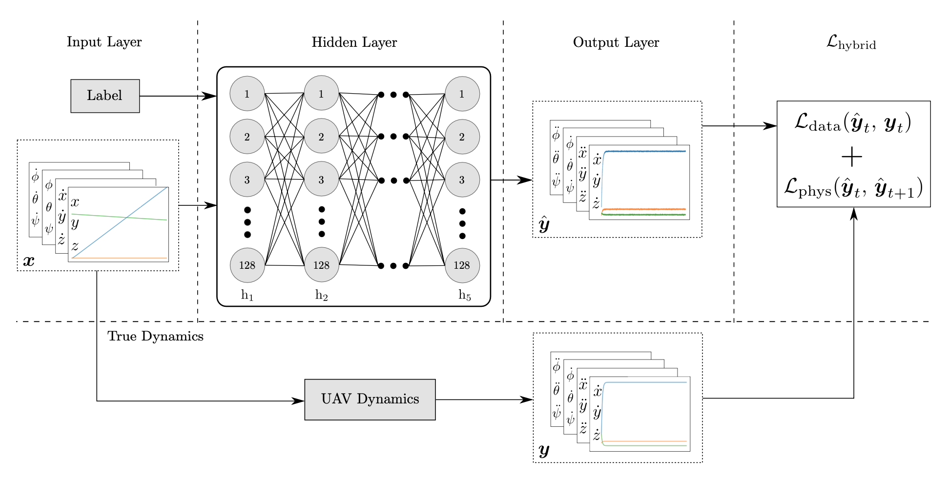
This work addresses object identification under known dynamics in UAV applications, where learning and classification are combined through a physics- informed residual neural network (PIRNN).
Quadcopter, fixed-wing, and helicopter aerial vehicles are considered as case studies.
Source code available on GitHub.
See the expanded description below.
Read more …
Methodology
- Network Architecture
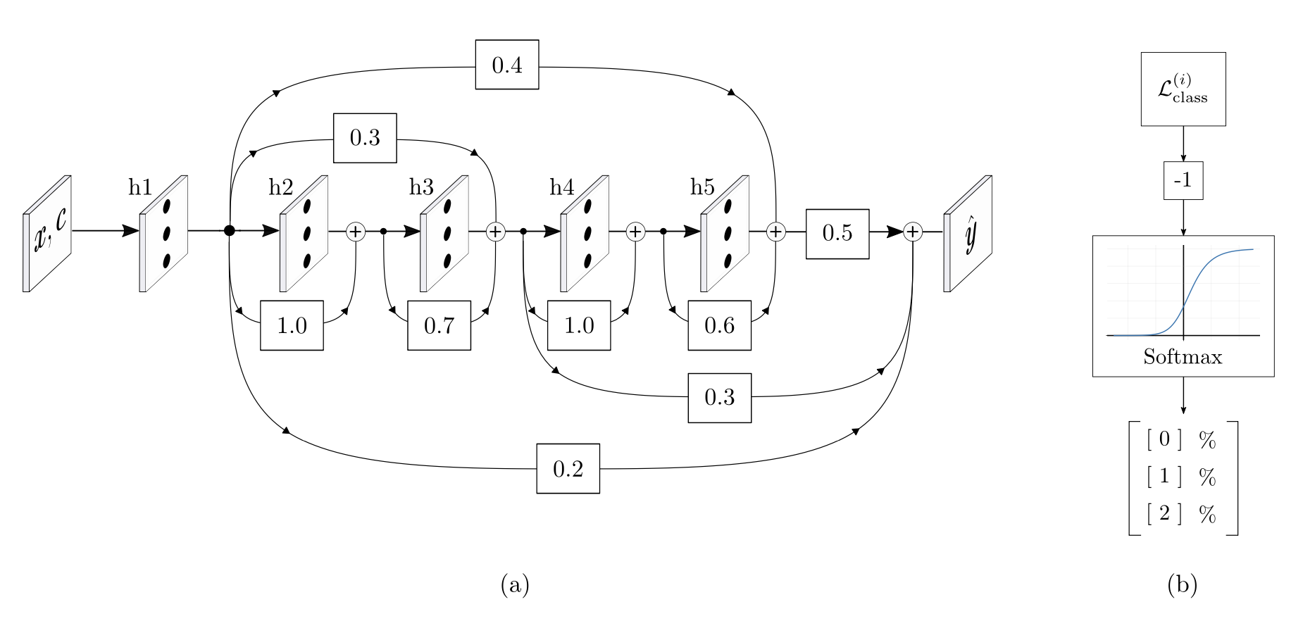
(b) Softmax-weighted Multi-class Confidence Estimation
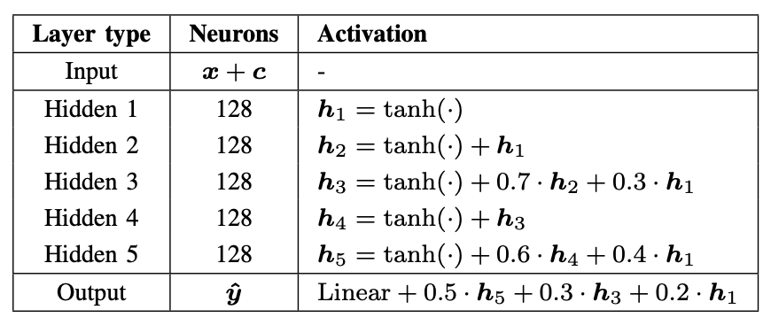
- Loss Function Design
Prior physical knowledge is integrated into the loss function.
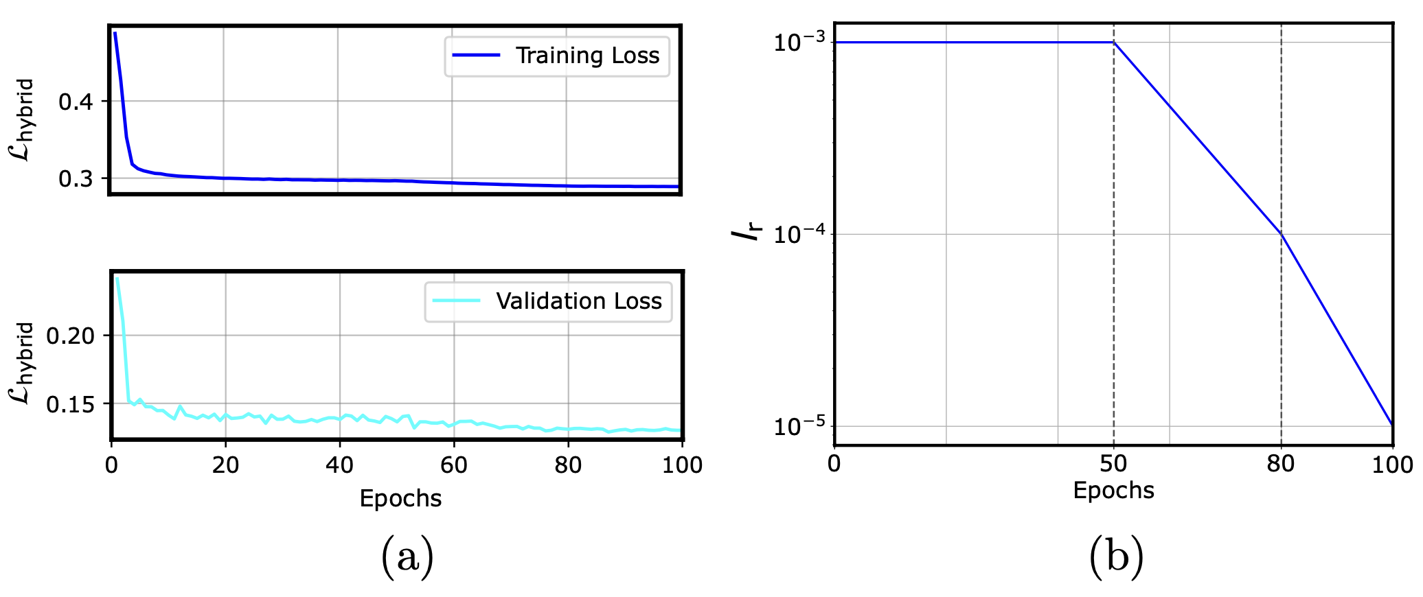
The hybrid loss function is designed to train the neural network to approximate the ground truth by minimizing the discrepancy between predicted and measured values, while simultaneously penalizing abrupt variations in state derivatives to enforce physical consistency.
- Softmax-Weighted Confidence Estimation for Multi-Class Classification
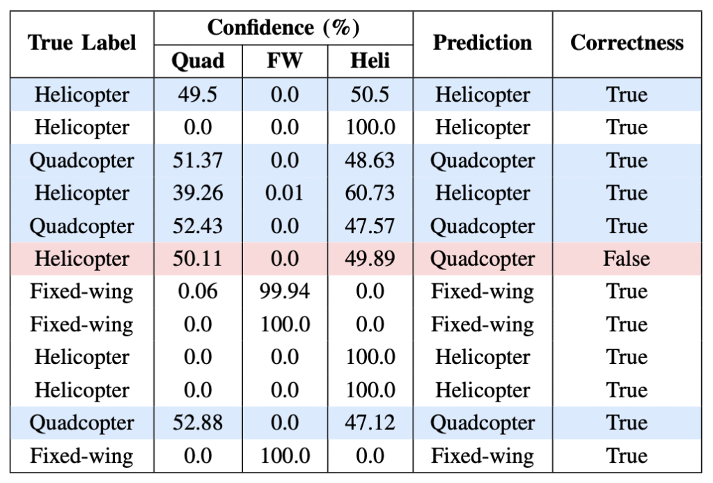
The resulting loss values are used to compute confidence scores via a softmax function. To ensure that lower loss values correspond to higher confidence scores, the losses are negated before being passed into the softmax operator σ(·), yielding a normalized distribution that sums to 1.
- Modeling and Dynamic Characteristics of UAV Types

Results
Reinforcement Learning-based Direct Torque Control of Externally Excited Synchronous Motors: a Proof of Concept
This paper is a revised and extended version of my master’s thesis and was published at the 2025 IEEE International Electric Machines & Drives Conference (IEMDC), Houston, Texas, USA.
This section corresponds to the original version of my master’s thesis, titled “Optimal Torque Control of Externally Excited Synchronous Motors by Reinforcement Learning.”
Both the IEEE paper and the thesis document are accessible by clicking their respective titles.
Source code available on GitHub.
See the expanded description below.
Read more …
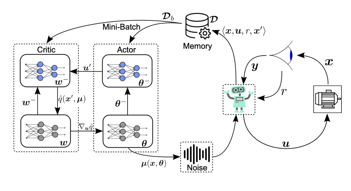
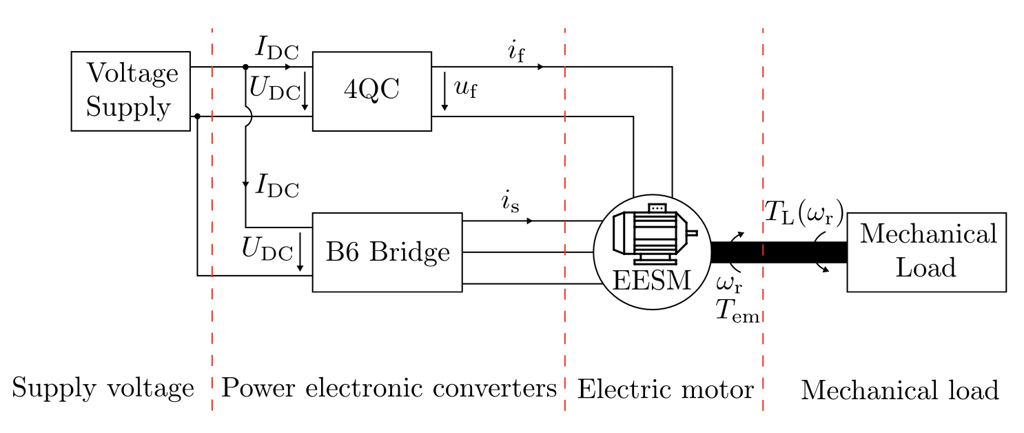
Since externally excited synchronous motors (EESMs) are a viable alternative to permanent magnet synchronous motors (PMSMs), they offer an additional degree of freedom through the excitation current. However, this advantage comes at the cost of strong cross-coupling between the d- and q-axes, which makes optimal control challenging. This project achieves optimal torque control using reinforcement learning through appropriate reward function design. The project is organized into five steps, corresponding to five work packages (WP01–WP05). Each work package corresponds to its own chapter or section in the thesis.
WP01: Overview of the System

WP02: CCS Current Control
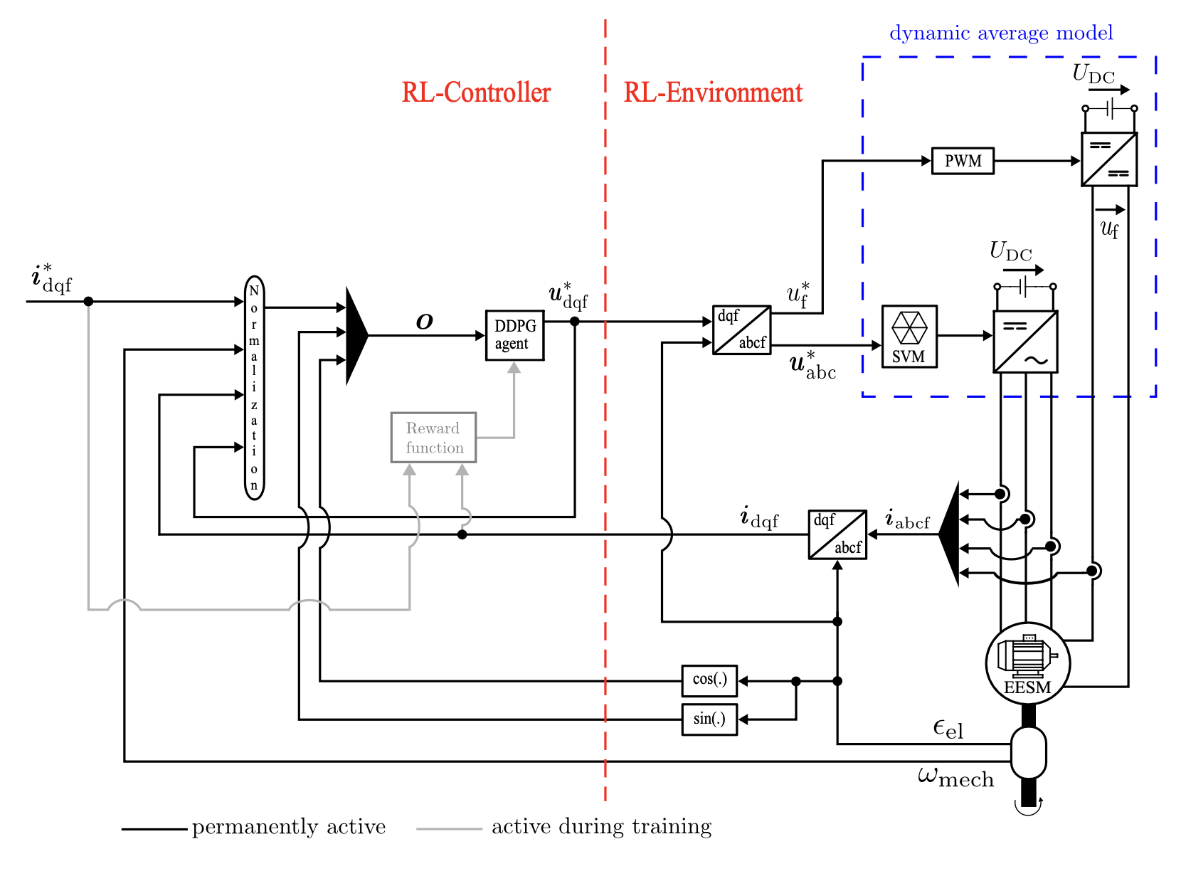
This analysis is conducted to demonstrate that the DDPG agent is capable of effectively navigating the complex, multi-dimensional control space of the EESM under a continuous control set.
This is critical for optimal torque control because, in real-world applications, torque sensors are typically unavailable, and current measurements serve as the primary feedback signals
Reward Design for CCS Current Control
1. Excess rotor current region
2. Excess stator current region
3. Unfavourable rotor current region
4. Tracking the references
Results
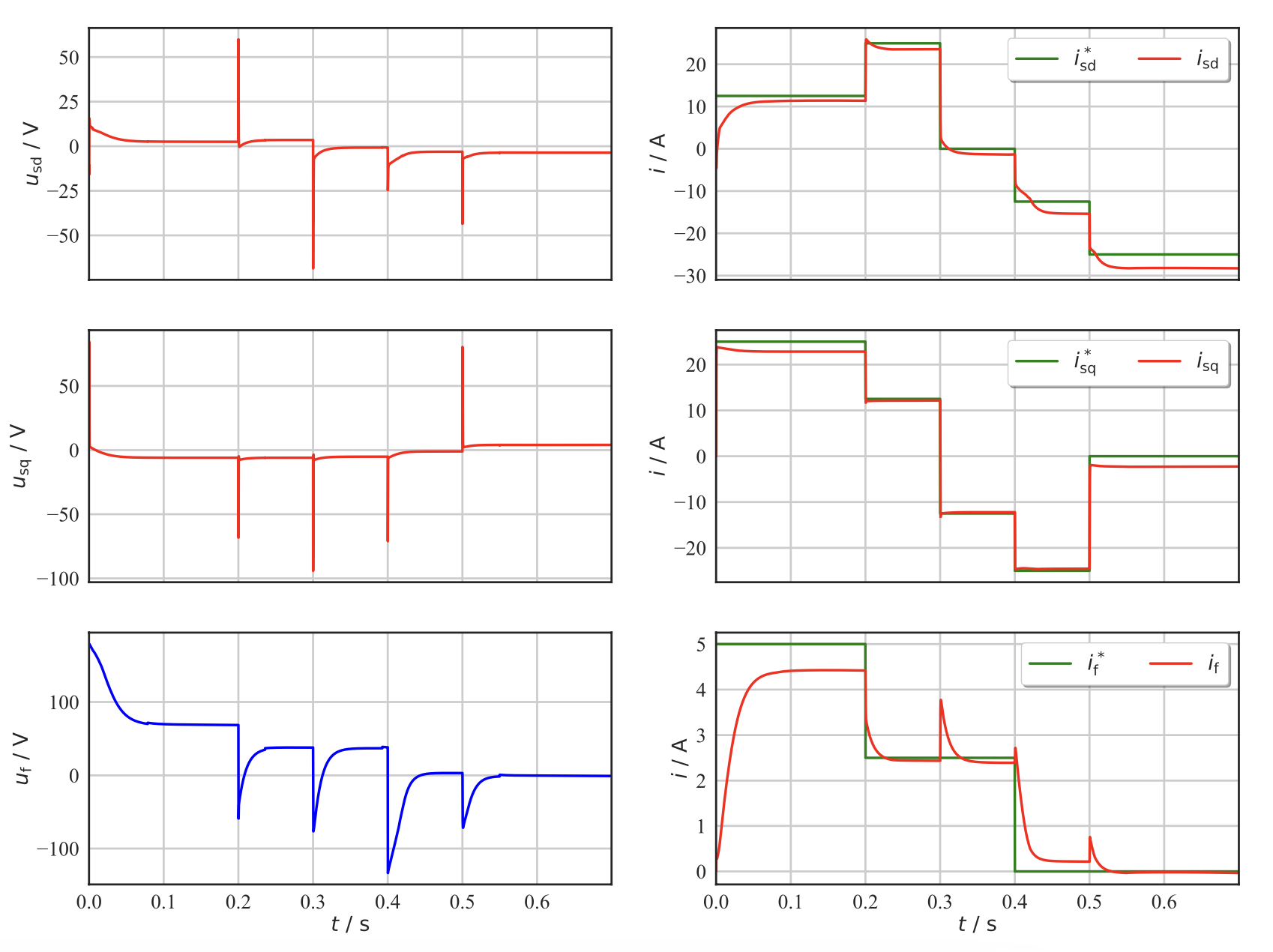
The DDPG agent effectively controls the d-, q-, and f-axes currents by applying the corresponding actions, addressing the challenges posed by the strong coupling effects between axes and the longer rotor time constant.
WP03: Torque Control with Idealized Excitation Circuit Current Control
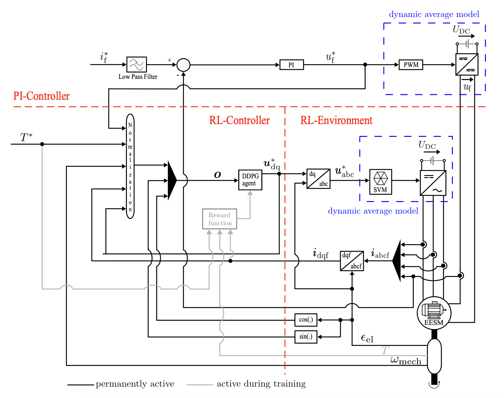
A PI-assisted RL controller was employed to facilitate a smooth transition from current control to torque control. The primary focus was on adapting the PMSM reward design to enable the EESM to behave similarly to a PMSM under constant excitation current conditions.
Reward Design for PI-assisted RL Control
1. Excess current region, E
2. Short-time over-current region, D
3. Unfavorable efficiency region, C
4. Desired operating region, B
5. Reference torque isoline, A
Visualization of Reward Design
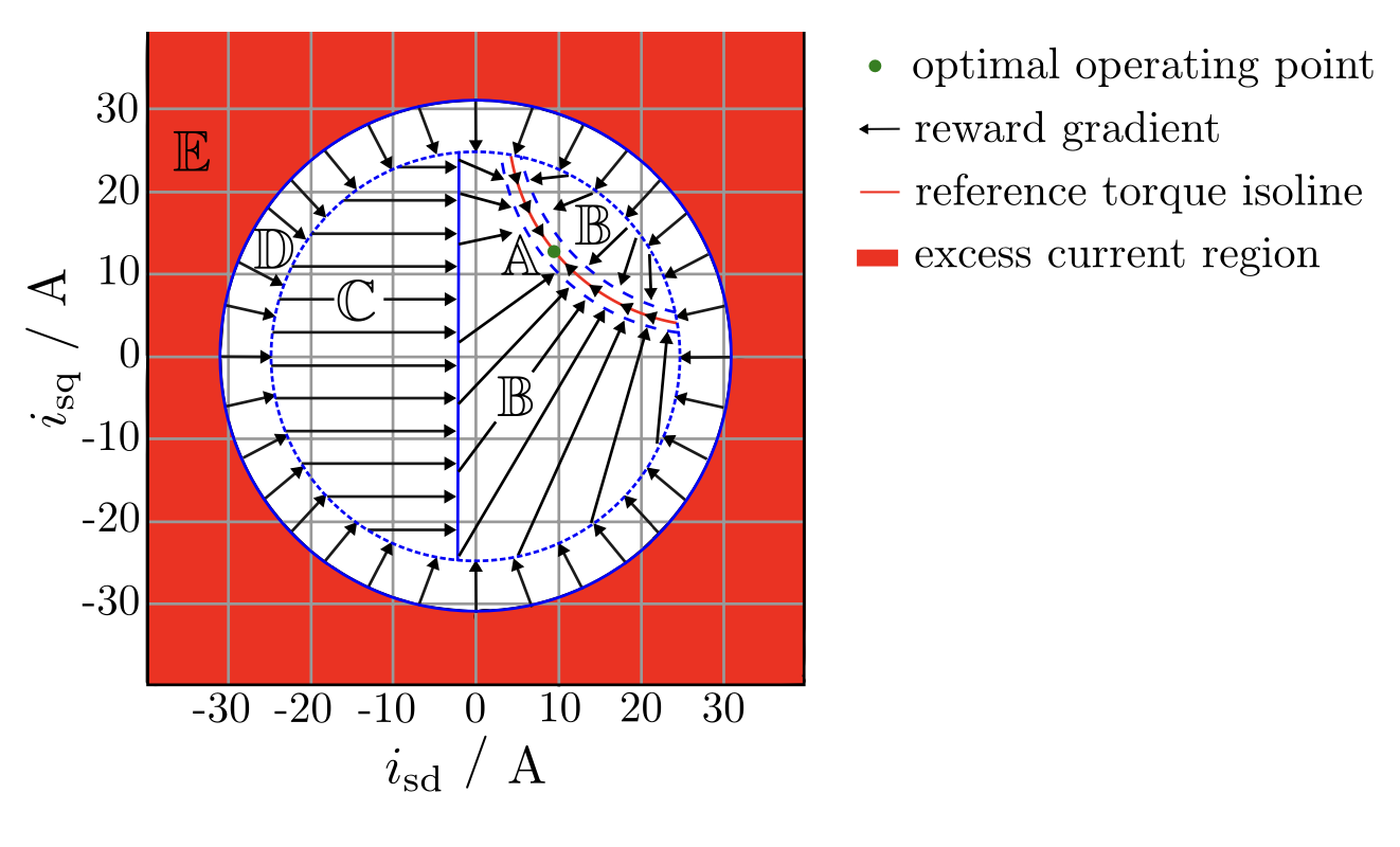
Results
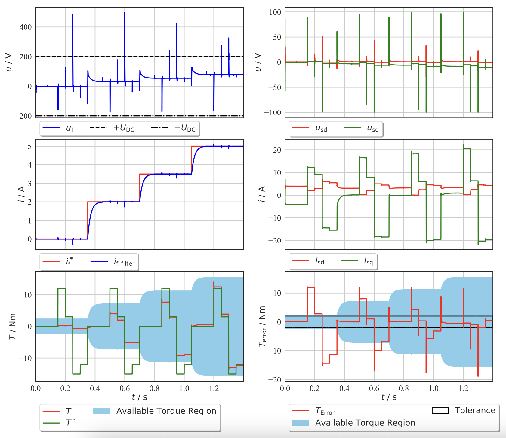
To this end, an idealized environment was created by removing the excitation voltage limit and employing a high working bandwidth for the PI controller.
Although this setup is not realistic for physical implementation, it provides valuable insights for future work. Specifically, the results indicate that an RL agent can manage the complex dynamics of an EESM for torque control, track the reference torque by manipulating stator current, and adapt to changes in excitation current, even when it is not controlled by the agent.
WP04: Torque Control with Reinforcement Learning based Excitation Circuit (Performance Priority Control)
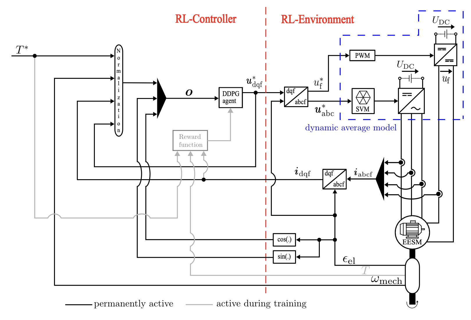
To ensure a smooth transition from the PI-assisted RL control to a fully RL-based control structure, the reward design from the previous section will be applied, with updates only to the safety constraints.
This approach allows the DDPG agent the flexibility to adjust the field current as needed, as long as it effectively tracks the reference torque.
Reward Design for Performance Priority Control
1.1: Region E in stator circuit
1.2: Region E in rotor circuit
2.1: Region C in stator circuit
2.2: Region C in rotor circuit
Visualization of Reward Design
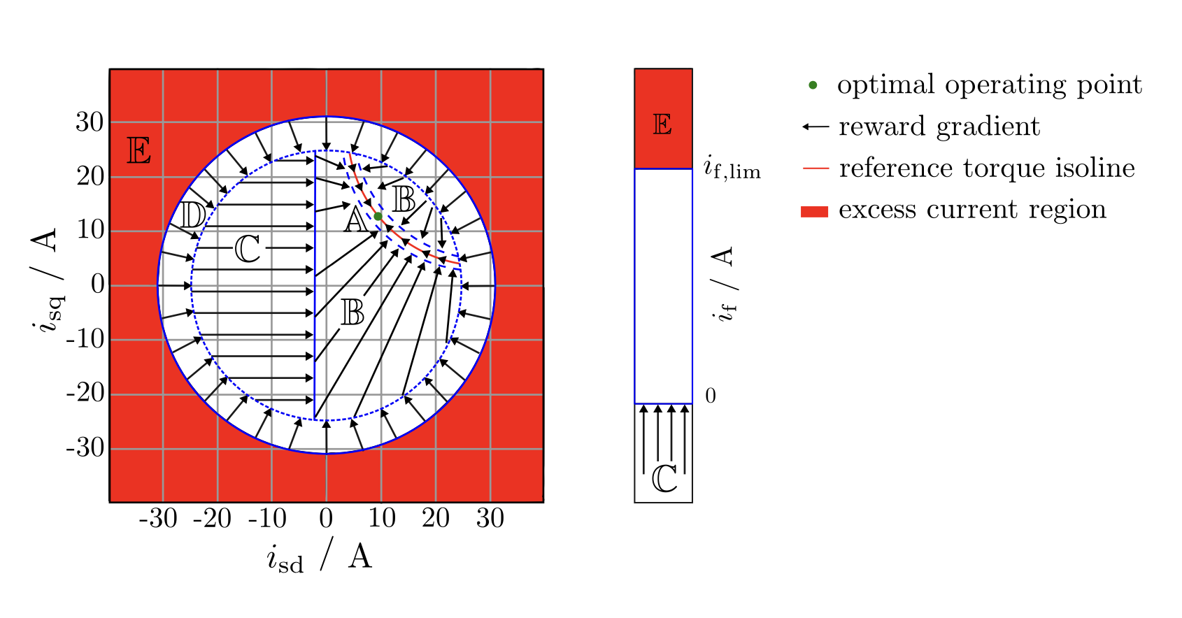
Apart from updating these two regions, the remaining regions (A, B, D) will retain the same design as before. Similarly, the prioritization of operating regions remains unchanged, with region A being the least important and region E the most important concerning the safety.
Results
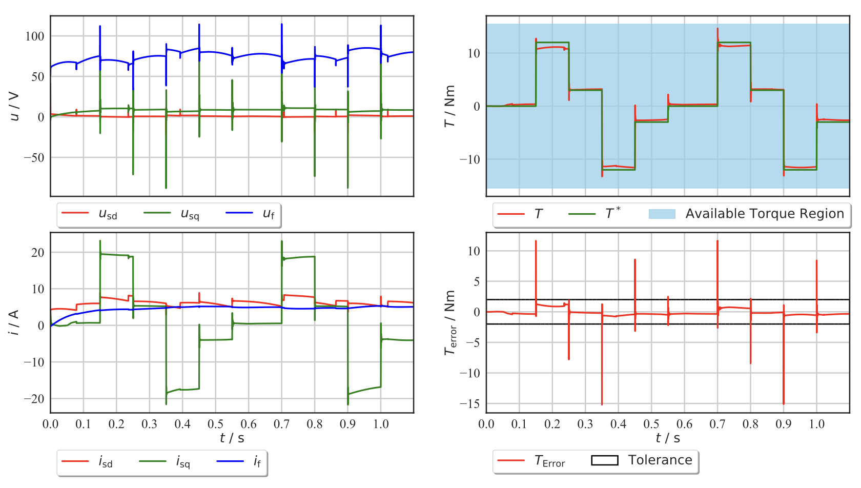
The agent adapts well to the changes in an environment, as it successfully tracks the reference torque with an error below the predefined tolerance. It is important to note that the available torque region remains nominal throughout the analysis, as the agent is allowed to apply the excitation current freely, as long as it is within the safety region.
WP05: Torque Control with Reinforcement Learning based Excitation Circuit (Efficiency Priority Control)
The schematic of the overall CCS torque control structure remains the same as shown above, while the efficiency calculation is incorporated into the reward design for Region A.
Efficiency enhancement in region, A
Both motor and generator operating modes are considered in the efficiency calculation.
Insight to Efficiency
Results
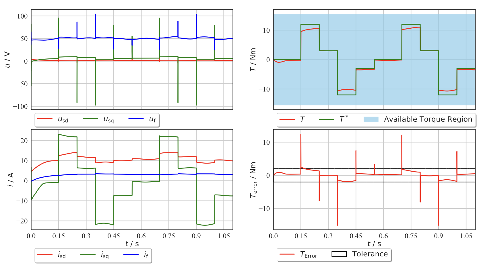
Two distinct strategies were explored: performance priority control and efficiency priority control. Each approach offers unique advantages, making the choice between them contingent on the specific requirements of the application.
For applications where precise torque tracking with minimal error is paramount, performance priority control is the preferred strategy. Conversely, if the application allows a broader error tolerance, efficiency priority control proves to be more beneficial.
Intelligent PID Control Augmented with Input Shaping for Precision Motion Control in Dynamic Systems
This paper has been submitted to the 2026 American Control Conference (ACC), New Orleans, LA, USA, and is currently under review. Any updates will be reflected here accordingly.
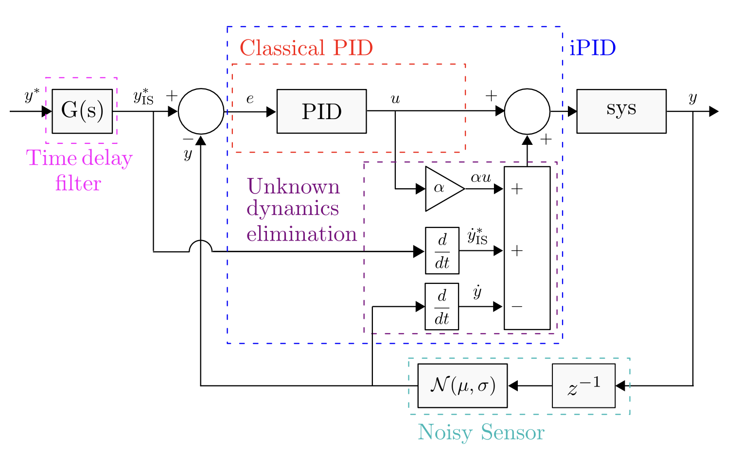
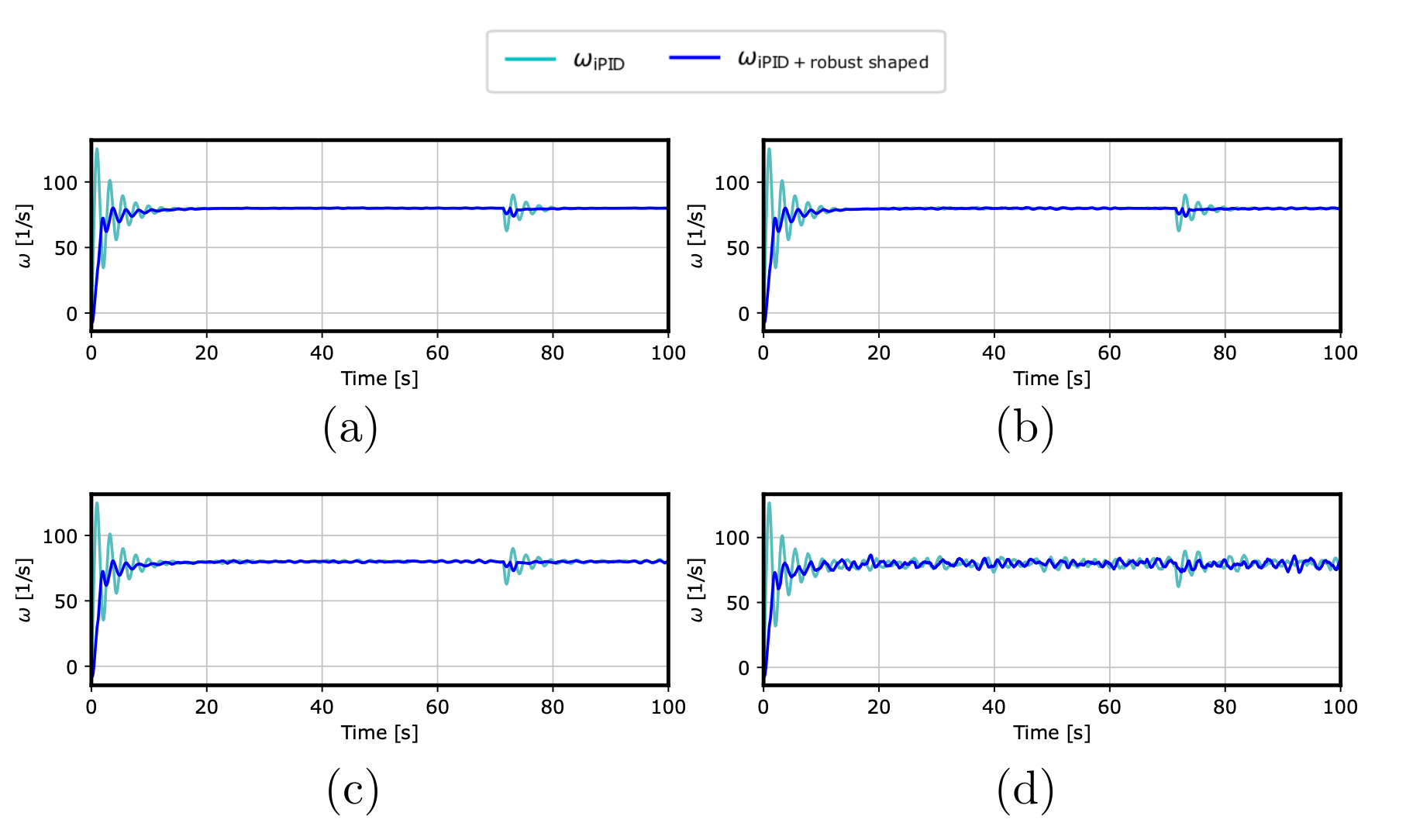
This work presents a model-free control frame-work that integrates an intelligent PID controller with input-shaping techniques to improve trajectory tracking in uncertain, noisy and vibration-prone systems.
The full paper will not be publicly accessible until the ACC 2026 review decision is released
Source code available on GitHub.
See the expanded description below.
Read more …
The iPID controller compensates for unknown dynamics, while input shaping suppresses residual oscillations without requiring detailed modeling.
Methodology
iPID Framework
Input Shaper Design
Benchmark Systems


Results
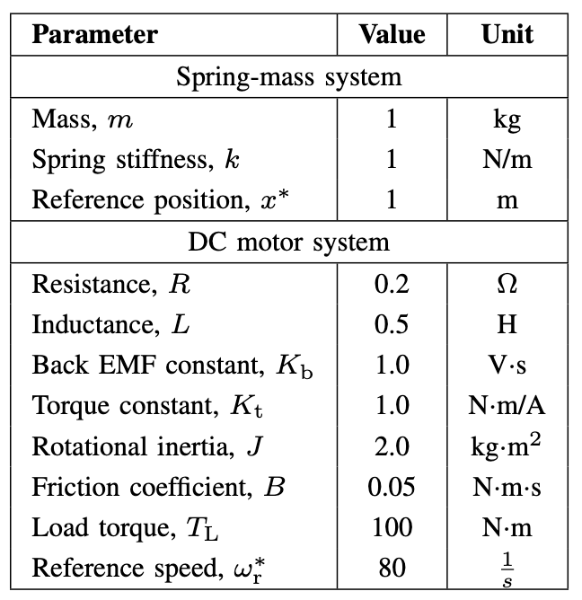
Only partial results of the DC motor system are presented here. The complete results will be made available after the paper is published.

Adaptive Input Shaper Design for Unknown Second-Order Systems with Real-Time Parameter Estimation
This is my second paper submitted to the 2026 American Control Conference (ACC), New Orleans, LA, USA, and it is currently under review. Any updates will be reflected here accordingly.
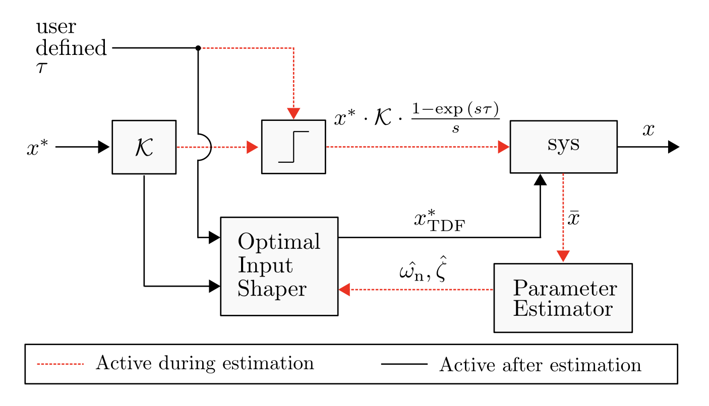
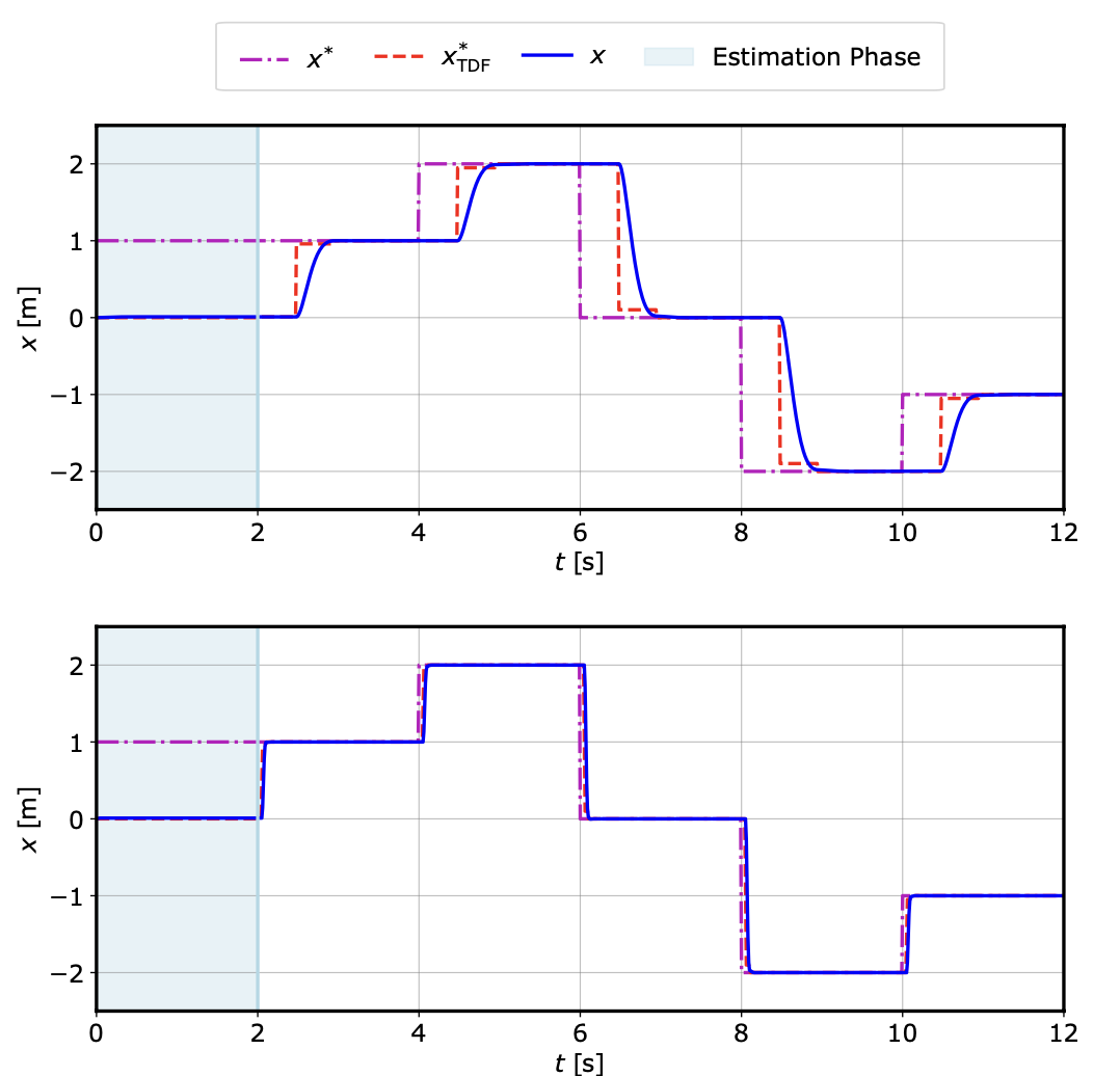
This work addresses the problem of designing an input shaper for an unknown system, where the switch time is highly sensitive to the system’s natural frequency. A feedforward control method is proposed that not only estimates system parameters online for a black-box second-order system, but also designs the input shaper adaptively in real-time.
The full paper will not be publicly accessible until the ACC 2026 review decision is released
Source code available on GitHub.
See the expanded description below.
Read more …
Methodology
Parameter Estimation in Feedforward Control
Arbitrary Estimation Time for Closed Form Input Shaper
The equations for this section will be added after the paper is published.
Results
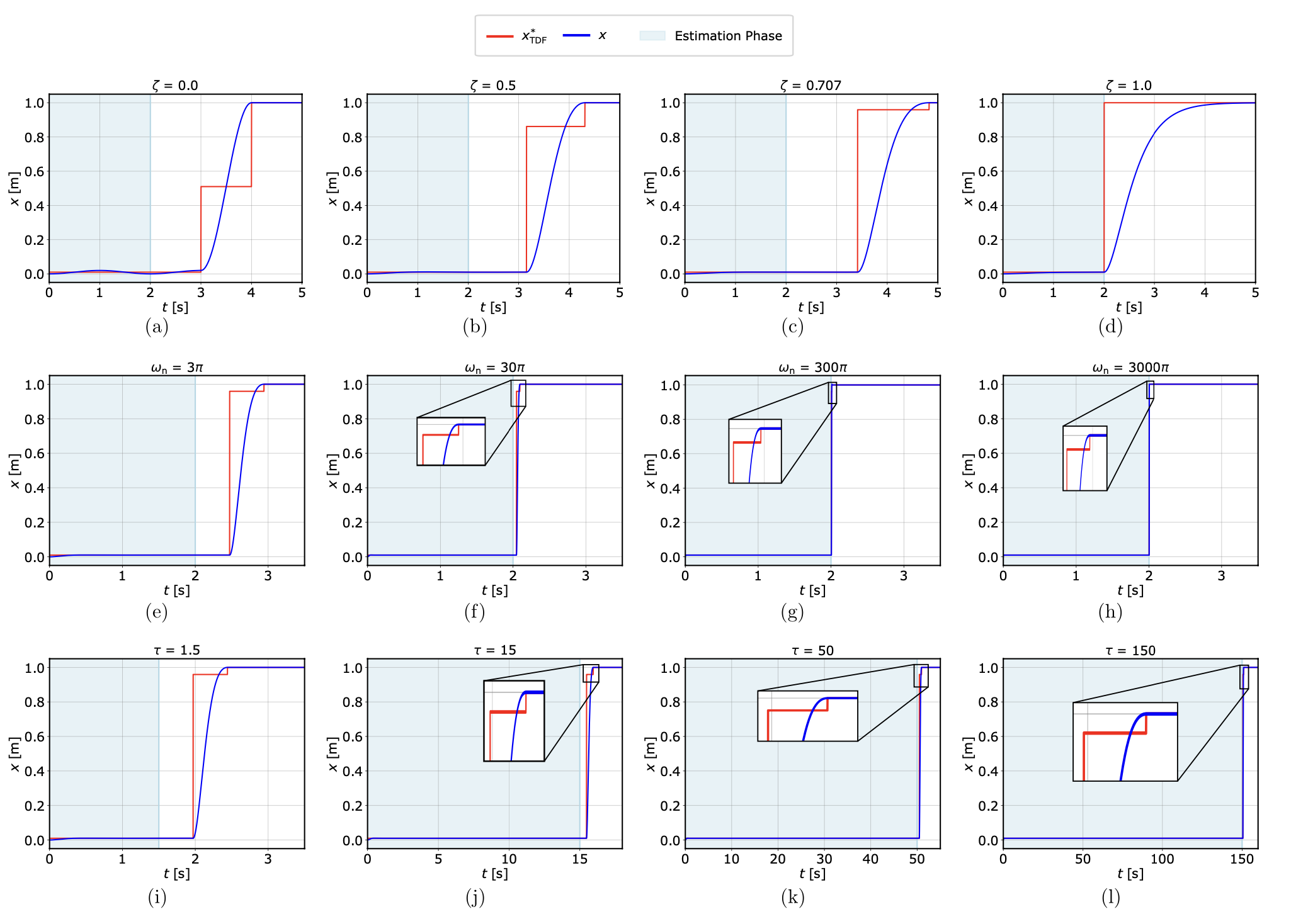
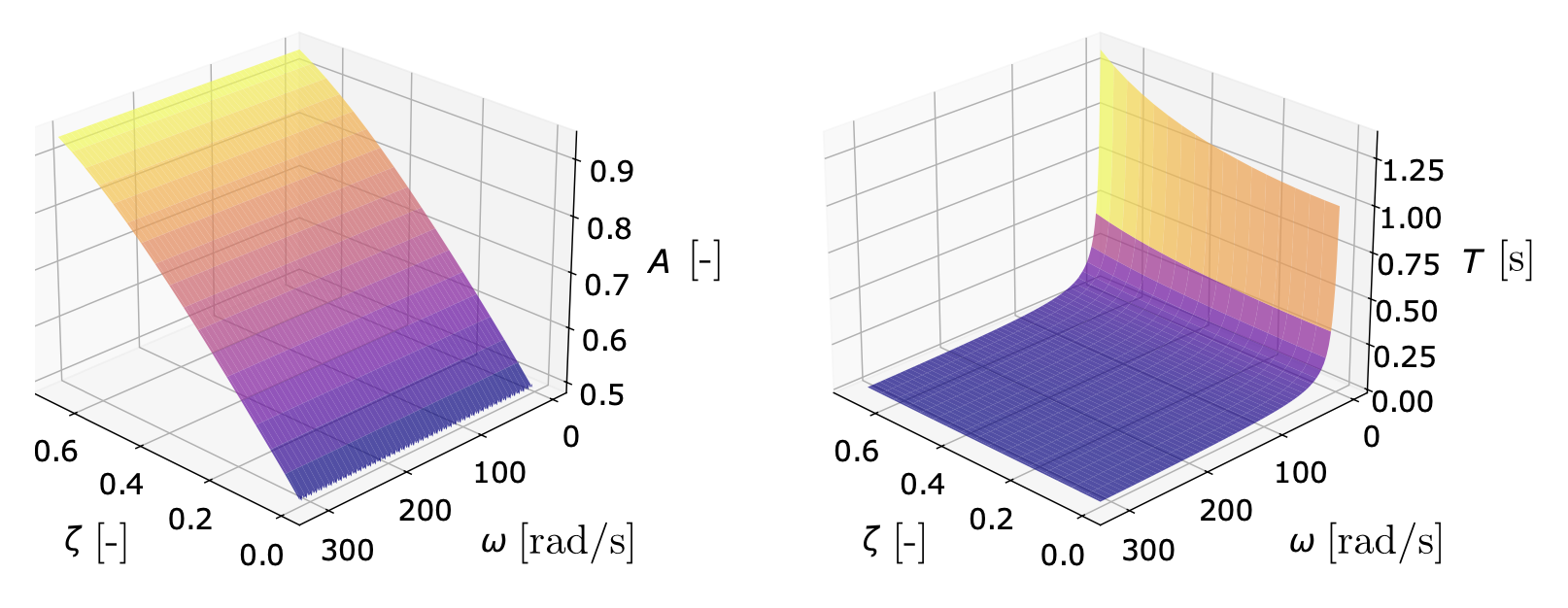
(a-d) varying ζ with τ = 2s and ω = π rad/s,
(e-h) varying ω with τ = 2s and ζ = 0.707,
(i-l) varying τ with ω = 3π rad/s and ζ = 0.707.
From Pixels to Patterns: Computer Vision Based Identification and Tracking of Liquid Metal Droplets
This project originated as coursework and is under active development, with the goal of being extended into a journal or conference paper.
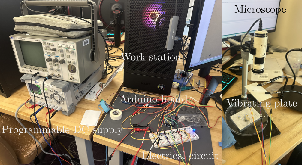
This work investigates the behavior of liquid metal droplets under vibration, with a particular focus on the breaking of their oxidized outer layer, which is critical for forming conductive pathways.
The behavior of liquid metal droplets under applied vibration is captured using a digital microscope. The recorded video frames are then processed using image processing techniques, including compression with discrete cosine transform and reconstruction via inverse discrete cosine transform, along with denoising, adaptive histogram equalization, edge detection, and contour extraction.
Source code available on GitHub.
See the expanded description below.
Read more …
Methodology
Since this work is still in progress, the detailed equations are omitted and will be added after the paper is published.
Image Preprocessing
- DCT and IDCT
- Denoised Convolutional Neural Network
- Contrast Limited Adaptive Histogram Equalization
Motion Detection
- Edge Detection
- Morphological Transformations
- Feature Extraction
- LM Droplet Characterization
Results
Detailed results and analytical conclusions will be reflected here at a later stage.

(a,c) The initial state with inconsistent or separated droplets before vibration;
(b,d) Droplet deformation and merging after vibration is applied.
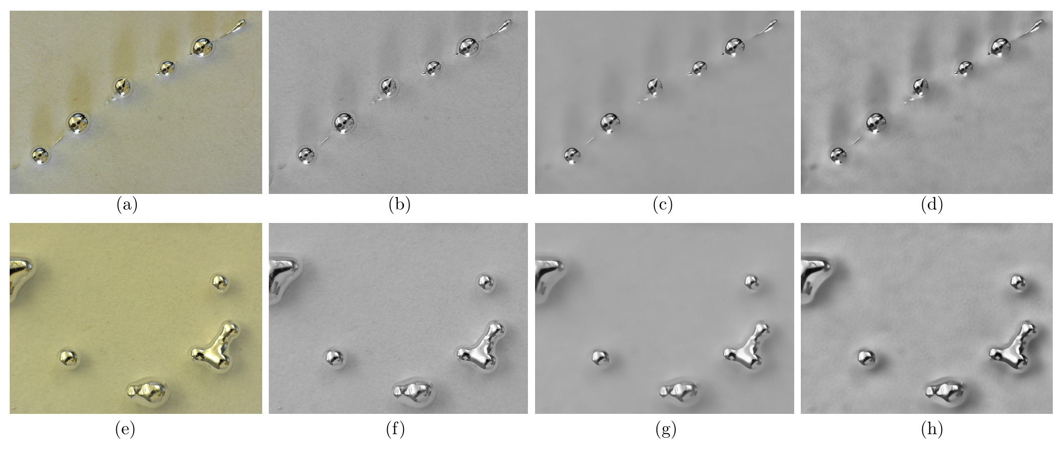
(a,e) Original frames; (b,f) Grayscale conversion followed by DCT and IDCT to suppress high frequency components; (c,g) Denoising using DnCNN by removing the estimated noise; (d,h) Contrast enhancement applied to highlight droplet boundaries and improve separation from the background.

Open-Loop Speed Control of Induction Motor
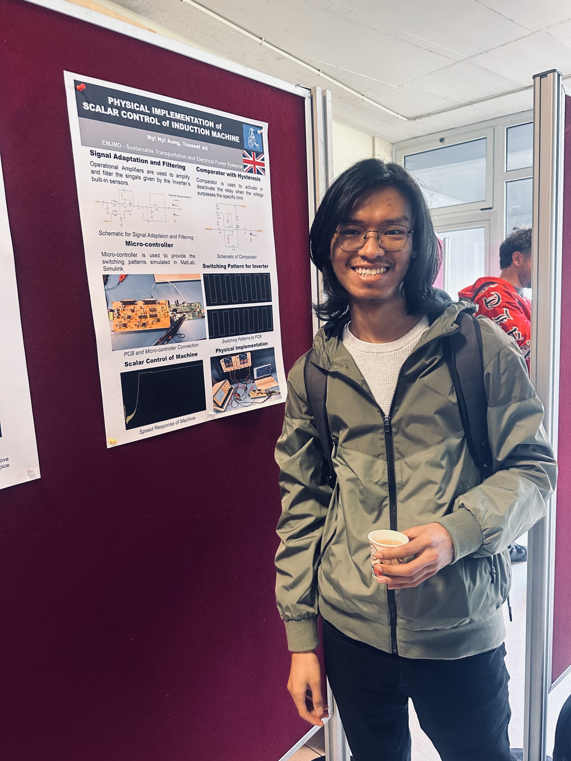
This project was carried out by my colleague Touseef and me during our master’s studies at the University of Oviedo, Spain, and was presented as an internal university poster.
Read more …
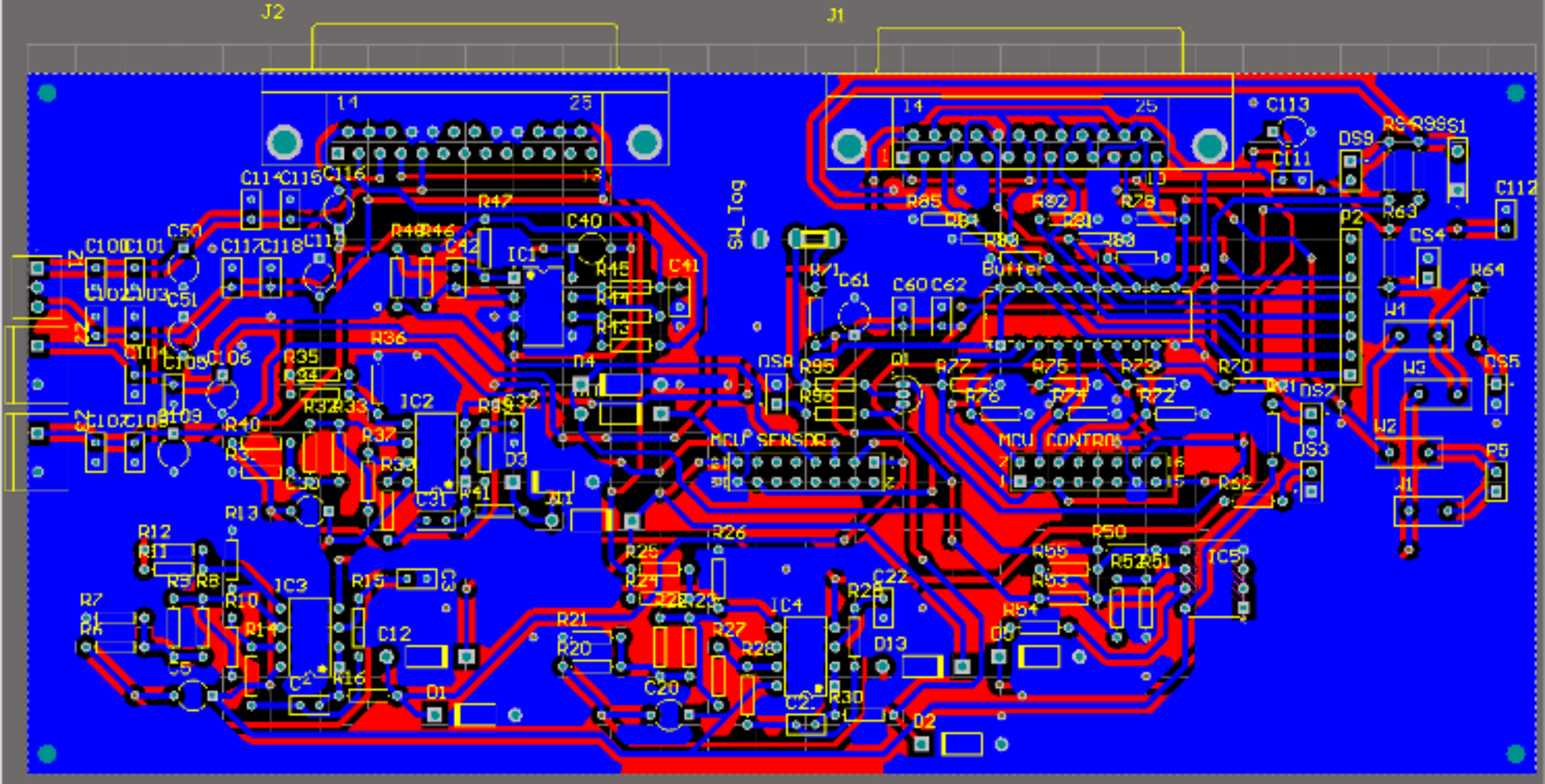
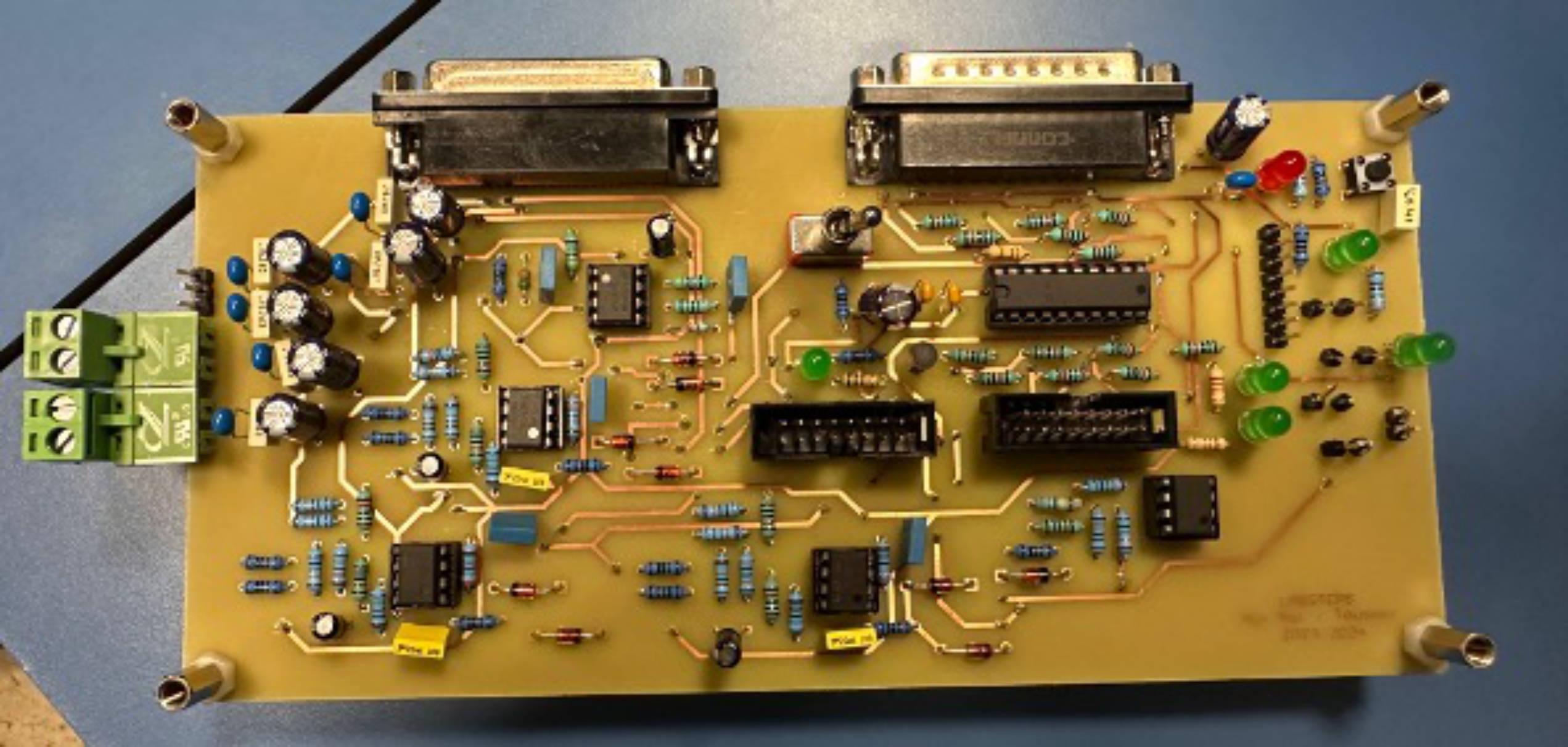
In this project, I gained hands-on experience working with operational amplifiers for signal amplification and filtering of measurements from the inverter’s built-in sensors, as well as comparators used to activate or deactivate a relay when the voltage exceeds a specified threshold.
The figures below show my PCB design and physical implementation.
Battery Charging through HB-LLC Resonant Converter
This project was conducted during my master’s studies. Although I did not have the opportunity to further develop an extended version, it represents a substantial amount of effort and learning, and I therefore include it here as part of my academic work.
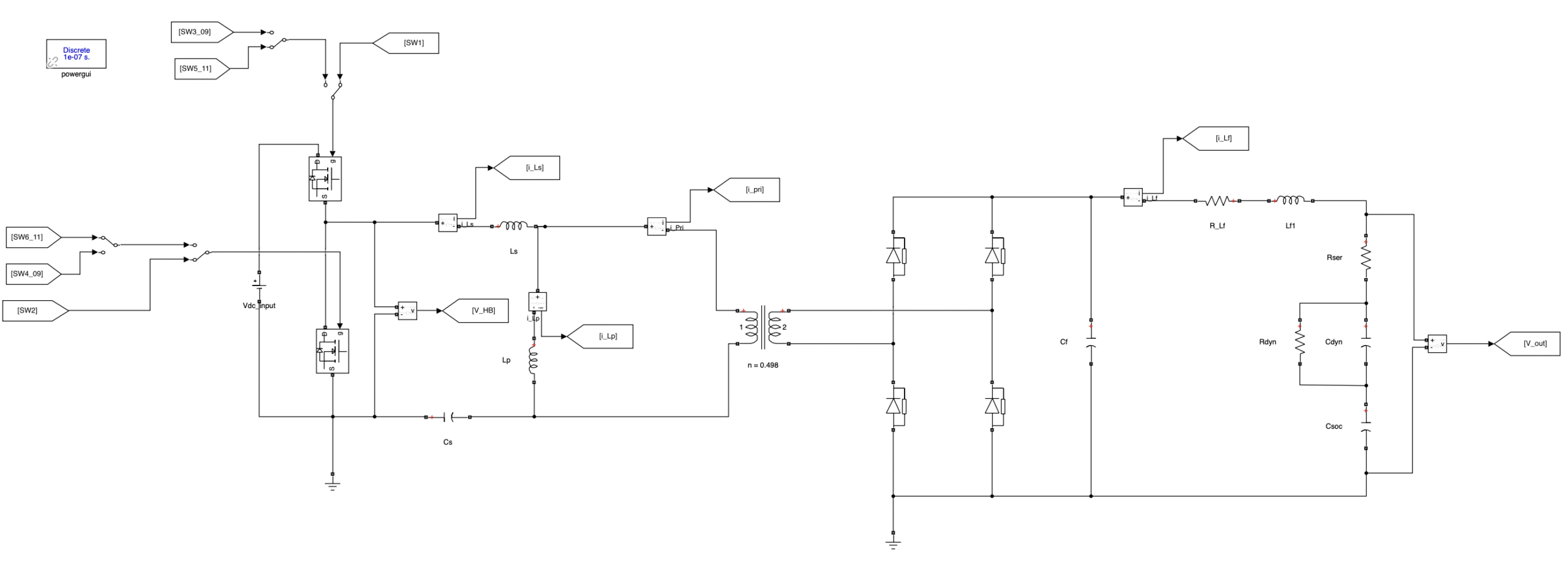
This project includes battery modeling, design and modeling of an HB LLC resonant converter, analysis of different switching patterns to investigate resonant, inductive, and capacitive switching behaviors, and the design of PI controllers for constant-current and constant-voltage charging.
Read more …
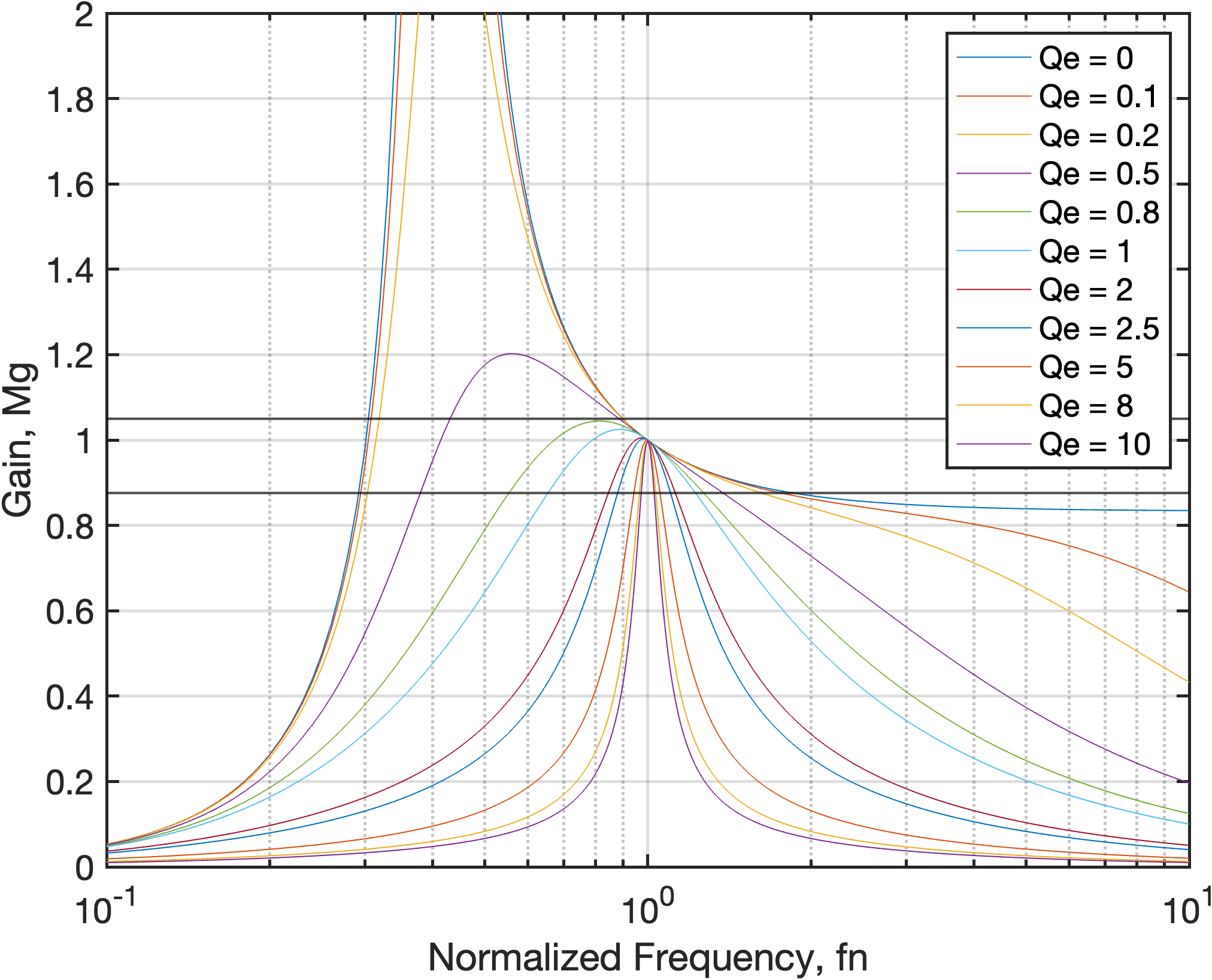
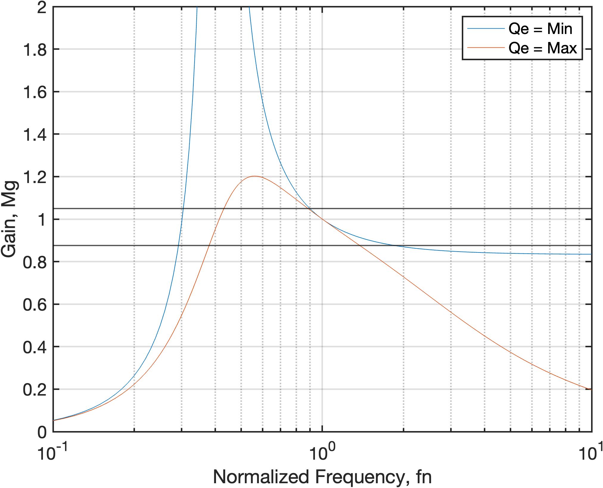
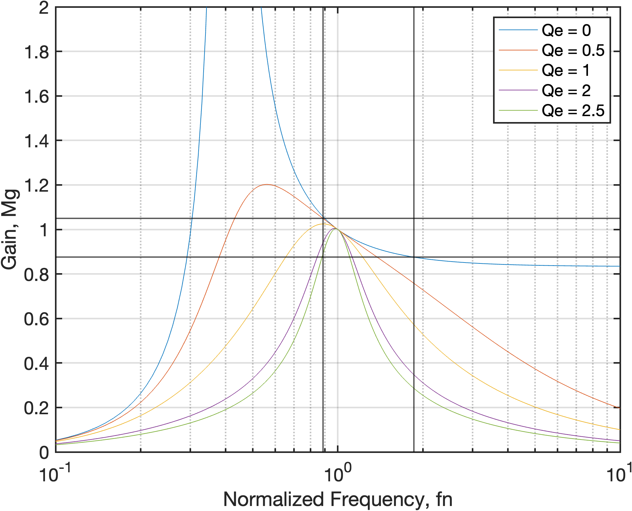
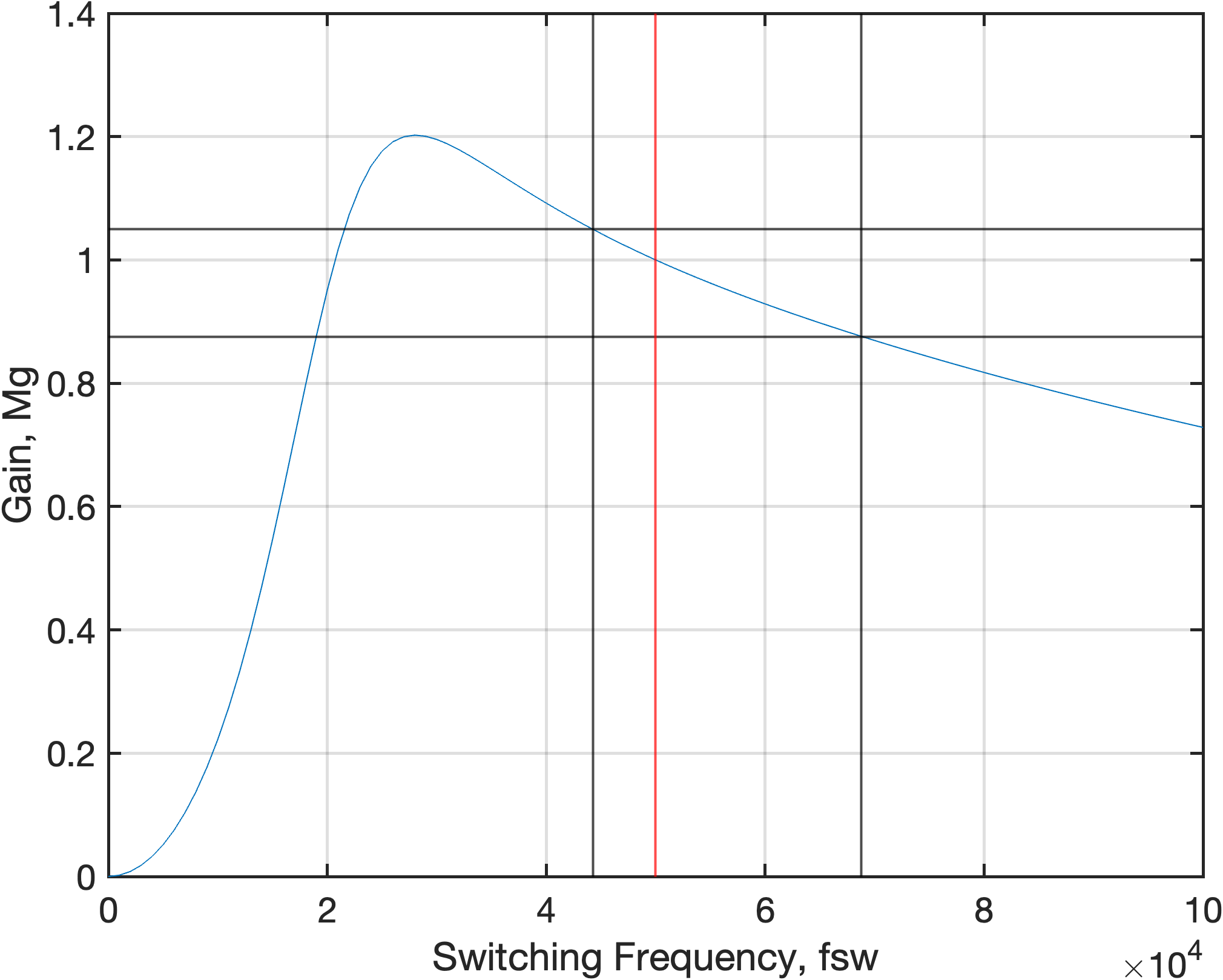
Resonant Tank Design
An inductance ratio of 5 is considered in this project.
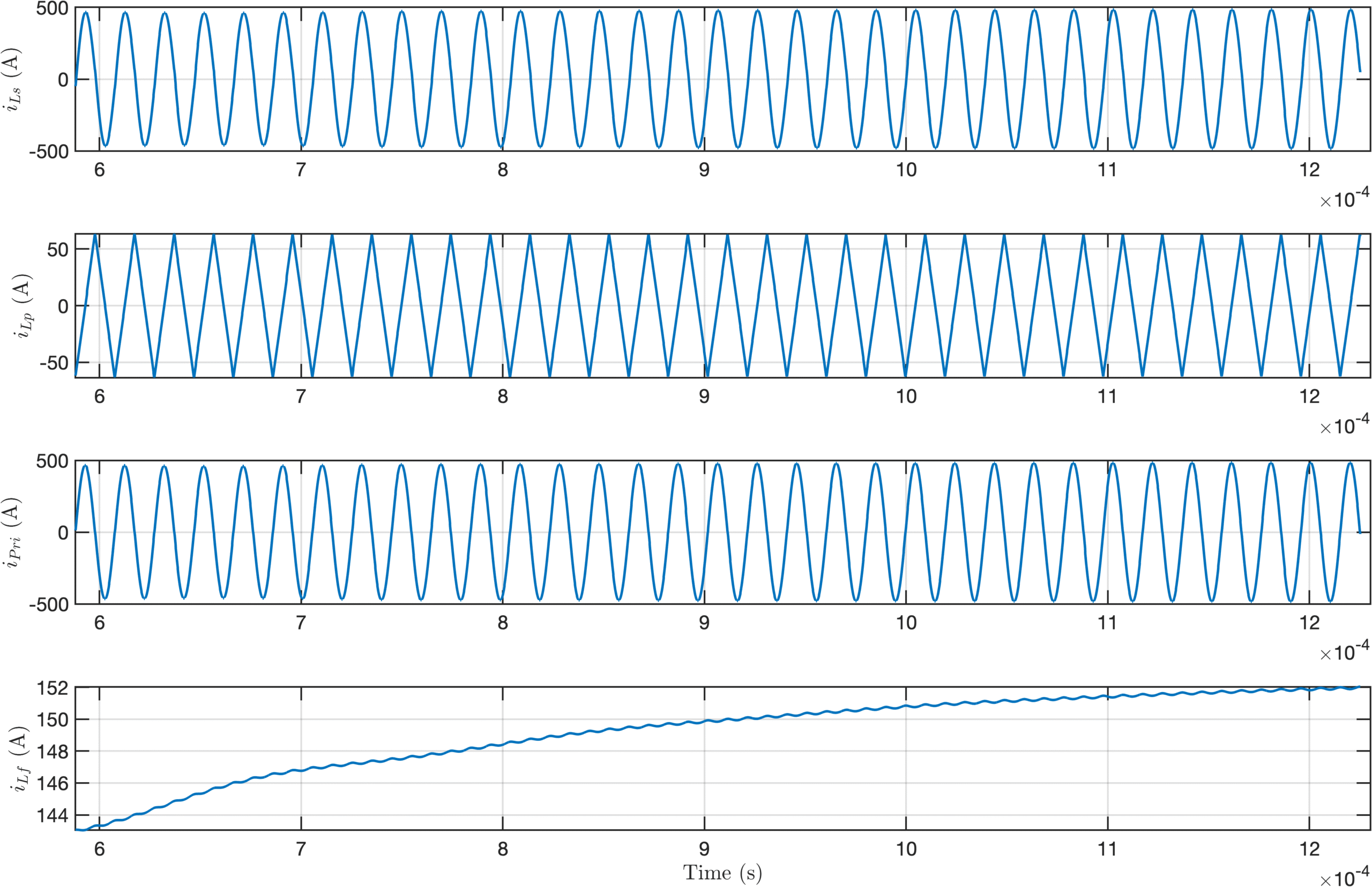
Resonant Tank Current Behavior Under Resonant Switching
Inductive and capacitive switching behaviors are difficult to observe visually and require significant zooming. Therefore, only the resistive switching behavior is shown here.
Due to time constraints, this page currently focuses on the modeling and design of the converter and battery, controller design will be included in a future update.

